Introduction to Deep Learning

Deep learning, a training method that combines computing power and data, has been widely used since the use of GPUs to train AlexNet on ImageNet in 2012.
We need to understand what deep learning is and how it differs from traditional machine learning.
Deep learning is a combination of deep neural networks and architecture = deep learning models.
Although deep learning is highly effective, its interpretability is poor and it is currently almost a black box.
Deep learning relies on the amount of data available. For real-world tasks, if data is insufficient, it is best not to use deep learning to train from scratch, as this will result in performance inferior to traditional machine learning algorithms. Choose the most suitable model based on the size and distribution of the dataset.
Deep learning is non-convex, meaning that we may not find the theoretical “global optimal solution.” In practice, trained networks often reach local optimal solutions, but local optimal solutions in deep neural networks often perform well.
The primary optimization algorithm in deep learning is backpropagation.
In terms of scale and number of layers, neural networks with more than one layer are theoretically called deep neural networks (DNNs). In practice, there is no clear distinction.

Neural Network

A neural network is a combination of linear transformation and activation function.
Formula: $\mathbf{h} = \sigma(W \mathbf{x} + b)$
Without an activation function, a multi-layer model degenerates into a single-layer linear model.
The key to success in deep learning: nonlinear activation functions + stacking.
Common activation functions include: Tanh, ReLU, Sigmoid, Softmax, etc.
Currently, the Pytorch framework is generally used as a launchpad for training models in the deep learning field, while the TensorFlow framework is gradually fading from mainstream use.

Forward Propagation

Forward propagation simply involves input (usually converted to a matrix) -> linear transformation + activation function -> output.
Forward propagation does not involve gradient updates or parameter updates.

\[\begin{align*} z1 = W1x + b1 \\ a1 = σ(z1) \\ z2 = W2a1 + b2 \\ ŷ = σ_{out}(z2) \end{align*}\]

Back Propagation

Backpropagation is the most important optimization algorithm in deep learning.
When training neural networks, we generally use the chain rule to calculate the gradient of the loss function with respect to the parameters to update the weights.
The calculation process is generally forward to obtain the output $ŷ$ -> calculate the loss -> calculate layer by layer -> parameter update
Essence: propagate the error layer by layer and use gradient descent to optimize the parameters
Let’s take an example
1. Input Layer: $x$
2. Hidden Layer: $z^{[1]} = W^{[1]}x + b^{[1]}, \quad a^{[1]} = \sigma(z^{[1]})$
3. Output Layer: $z^{[2]} = W^{[2]}a^{[1]} + b^{[2]}, \quad \hat{y} = \sigma(z^{[2]})$
4. Loss Function: $L = \frac{1}{2}(y - \hat{y})^2$
Back Propagation step:
1. Output Error: $\delta^{[2]} = \frac{\partial L}{\partial z^{[2]}} = (\hat{y} - y) \cdot \sigma’(z^{[2]})$
2. Hidden Error: $\delta^{[1]} = \frac{\partial L}{\partial z^{[1]}} = (W^{[2]})^T \delta^{[2]} \cdot \sigma’(z^{[1]})$
Gradient Compute:
1. $\frac{\partial L}{\partial W^{[2]}} = \delta^{[2]} (a^{[1]})^T$
2. $\frac{\partial L}{\partial b^{[2]}} = \delta^{[2]}$
3. $\frac{\partial L}{\partial W^{[1]}} = \delta^{[1]} x^T$ $\frac{\partial L}{\partial b^{[1]}} = \delta^{[1]}$
The specific details of backpropagation are not explained. We only need to know that the goal of the neural network is to minimize the loss function. Without the backpropagation algorithm, using other algorithms (such as numerical algorithms) requires a complexity of $O(n^2)$. With backpropagation, we can achieve the same complexity as forward propagation, $O(n)$.
Without backpropagation, it is difficult to train large-scale neural networks.

Optimization Algorithms

Gradient Descent (GD) uses all samples to update parameters each time. It is very inefficient when the amount of data is large.
Stochastic Gradient Descent (SGD) uses one sample to update parameters each time. It is fast to calculate and can jump out of the local optimum, but it has large fluctuations and is not easy to converge.
Mini-batch Gradient Descent uses a small batch of samples (batch) to update parameters each time. It is a compromise between efficiency and stability.
Momentum $v = βv + (1-β)∇L θ = θ - ηv$ simulates inertia, reduces oscillations, and accelerates convergence.
Adagrad uses adaptive learning rates to reduce frequent learning rate updates, but its drawback is that small learning rates can lead to premature stagnation.
RMSProp uses weighted averaging to improve the rapid decay of Adagrad’s learning rate.
Adam (Adaptive Moment Estimation) combines momentum with RMSProp and is the most commonly used optimizer.
AdamW introduces weight decay to Adam, resulting in more stable results and is a commonly used optimizer for LLM.
Others: AdaMax, Nadam, LAMB, MuonClip, etc.

Regularization Methods

Regularization methods are generally used to prevent model overfitting and improve robustness and generalization.
Regularization methods are generally categorized into L1 and L2, dropout, data augmentation, early stopping, batch normalization, and layer normalization.
L1 is Lasso, which makes the parameters sparse: $\lambda\sum_{i} \lvert wi \rvert$
L2 is Ridge, which makes weights smaller but not sparse: $\lambda\sum_{i} \lvert wi \rvert$
Dropout randomly drops neurons during training.
Data Augmentation modifies the model to make it more robust. Methods include rotation, translation, flipping, and adding noise.
Early Stopping monitors the loss and stops training if performance starts to decline.
Batch Normalization/Layer Normalization normalizes the outputs of intermediate layers to reduce exploding and vanishing gradients. A small amount of regularization is more like an optimization technique.
Why are Regularization Methods rarely used for training LLMs? LLMs require a very large amount of data and often suffer from underfitting. Furthermore, optimizers like the AdamW optimizer use a small amount of regularization and weight decay.

Initialization Methods

Keep the activations and gradient variances of each layer as stable as possible during forward and backward propagation to prevent vanishing and exploding gradients, making it easier to train deep networks.
Random Initialization: Both Gaussian and uniform distributions are acceptable.
Uniform: $W_{ij}\sim \mathcal{N}(0,\sigma^2)$
Gaussian: $W_{ij}\sim \mathcal{U}[-a,a] \mathrm{Var}=a^2/3$
He Initialization (Kaiming Initialization)
LeCun Initialization
Xavier Initialization (Glorot Initialization), etc.

Convolutional Neural Networks (CNN)

CNN is the core model for processing grid data such as images, videos, and speech in deep learning.
Compared to fully connected networks, it has fewer parameters and better preserves spatial structure.
Convolutional neural networks were proposed by Le. Their general layer architecture is: convolution layer + activation function + pooling layer + fully connected layer + normalization layer.
The convolution layer performs a local weighted sum on the input feature map using a convolution kernel (filter/kernel).
$\begin{align*}y_{i,j,k} = \sum_{c=1}^{C} \sum_{m=1}^{M} \sum_{n=1}^{N} x_{i+m, j+n, c} \cdot w_{m,n,c,k}\end{align*}$
Parameters: kernel size (M×N), stride, padding
Activation functions: ReLU, Leaky ReLU, GELU, etc., which increase nonlinearity and can learn complex parameters from the data
Pooling layers: MaxPooling / AveragePooling, which reduce image size and computational complexity
Fully connected layers: After convolutional feature extraction, fully connected layers perform regression or classification
Norm layers: Perform normalization, add block convergence, and alleviate vanishing gradients
CNN Architectures: LeNet, AlexNet, VGGNet, ResNet, DenseNet, GoogleNet, etc.
The most important CNN architecture is ResNet. By introducing residual connections, it solves the vanishing gradient problem in deep neural networks. Formula: $y = F(x, {W_i}) + x$
CNNs are generally used for image classification, object detection, semantic segmentation, medical image analysis, etc.
CNN-derived architectures and algorithms include U-Net and YOLO.

Recurrent Neural Networks (RNN, GRU, LSTM)

These models are generally used for NLP, speech recognition, time series, video understanding, etc.
RNN
RNN, also known as recurrent neural network, is a neural network used to process sequential data (text, time series, speech, etc.).
Main Idea: Hidden State acts as memory, transferring historical information to the next moment.
RNNs are prone to problems such as vanishing/exploding gradients.
Improvements: GRU (Gated Recurrent Unit) LSTM (Long Short-Term Memory Network) $\text{Given $x_t$, Hidden state update: }\ h_t = \tanh(W_{xh} x_t + W_{hh} h_{t-1} + b_h)$ $\text{Output: }\ y_t = W_{hy} h_t + b_y$
GRU
Compared to RNNs, GRUs add memory cells (cell states) and gates, which effectively mitigate the vanishing/exploding gradient problem.
Can model long-term dependencies, but training is slow and requires a large number of parameters.
Input: $x_t$, Previous state: $h_{t-1}, c_{t-1}$
Input gate: $i_t = \sigma(W_{xi} x_t + W_{hi} h_{t-1} + b_i)$
Forget gate: $f_t =\sigma(W_{xf} x_t + W_{hf} h_{t-1} + b_f)$
Candidate Memory: $\tilde{c}_t = \tanh(W_{xc} x_t + W_{hc} h_{t-1} + b_c)$
State: $c_t = f_t \odot c_{t-1} + i_t \odot \tilde{c}_t$
Output Gate: $o_t = \sigma(W_{xo} x_t + W_{ho} h_{t-1} + b_o)$
Hidden State: $h_t = o_t \odot \tanh(c_t)$

LSTM

Alleviating vanishing/exploding gradient issues in RNNs during training and capturing long-term dependencies
Main Idea: Introducing Additive Cells The state $c_t$ and the gate $(i,f,o)$ allow the gradient to flow along $c_t$ almost “unimpeded.”
A simple reference implementation $\begin{bmatrix} i_t \\ f_t \\ g_t \\ o_t \end{bmatrix} = \begin{bmatrix} \sigma \\ \sigma \\ \tanh \\ \sigma \end{bmatrix} \left( W_x x_t + W_h h_{t-1} + b \right)$
Update the state $c_t = f_t \odot c_{t-1} + i_t \odot g_t$ $h_t = o_t \odot \tanh(c_t)$
$W_x \in \mathbb{R}^{4h \times d}$ , $W_h \in \mathbb{R}^{4h \times h}$, $b \in \mathbb{R}^{4h}$

Self-Supervised Learning

Before moving on to Transformers, we must first understand what self-supervised learning is.
Self-supervised learning (SSL) is a learning method that does not rely on human annotations.
Learning is achieved by constructing supervisory signals from the data itself.
SSL does not require human labels, but “pseudo-labels” are constructed during training.
SSL can be considered a combination of unsupervised and supervised learning.
Main idea: Design a pre-training task to construct “pseudo-labels,” for example, predicting masked words given a text sequence (BERT).
Representation Learning: Learn the feature space through these tasks.
Downstream tasks: Transfer the learned representations to tasks such as classification, regression, and generation.
Common methods:
Predictive SLL:

Masked Language Modeling (MLM, e.g., BERT)
Masked Autoencoder (MAE for vision)
Sequence Auto-regression (GPT)
- Contrastive SSL:
SimCLR, MoCo, BYOL, SimSiam
- Generative SSL
Autoencoder
Variational Autoencoder (VAE)
Diffusion-based SSL (e.g., Masked Diffusion Pretraining)

SimCLR (Chen et al., Google Research, 2020) is a self-supervised contrastive learning method that does not rely on labels and learns representations by maximizing the consistency of different augmented views.
InfoNCE Loss is:

\[\begin{align*} L_{\text{pre}}(\theta) = - \sum_{i=1}^{B} \log \frac{\exp \left( \phi_{\theta}(\hat{x}^{(i)})^{\top} \phi_{\theta}(\tilde{x}^{(i)}) \right)} {\exp \left( \phi_{\theta}(\hat{x}^{(i)})^{\top} \phi_{\theta}(\tilde{x}^{(i)}) \right) + \sum_{j \neq i} \exp \left( \phi_{\theta}(\hat{x}^{(i)})^{\top} \phi_{\theta}(\tilde{x}^{(j)}) \right)} \end{align*}\]

Transformer

As one of the most important model architectures in recent years, the Transformer has demonstrated excellent performance in tasks such as NLP, Computer Vision, and speech. This is especially true for the Generative Prediction (GPT) architecture derived from the Transformer.
I won’t go into detail about the Transformer architecture; there are excellent resources online cs336
In the 2017 Transformer paper, the core architecture is (Encoder+Decoder)
The core is Self-Attention+FFN+Residual+Norm
The Encoder extracts contextual information, and the Decoder autoregressively predicts the sequence.
The core of Attention: $\text{Attention}(Q, K, V) = \text{softmax}\left(\frac{QK^T}{\sqrt{d_k}}\right)V$
Modern LLMs are all decoder-only architectures, eliminating the original encoder and simplifying them to autoregressive language models.
As of August 2025, the typical combination of modern LLM architectures is RMSNorm+RoPE+FFN(SwiGLU)
LayerNorm+Learned has been replaced. Embedding + FFN (ReLU/GeLU)
Attention variants include new architectures like FlashAttention that optimize I/O and accelerate computation.
For a detailed introduction, see the CS336 lecture notes.
MoE (Mixture of Experts) architecture: Multiple FFN blocks are run in parallel, but only k experts are activated at a time. $y = \sum_{i \in \text{TopK}(G(x))} g_i(x) \cdot E_i(x)$
$E_i$ Experts(FFN)
$G(x)$ Gating network, determines which expert to route to
$g_i(x)$ Experts’ weights
Multimodal Transformer: Language + Vision + Audio + Code → Multimodal
Common architectures include single-tower, dual-tower, LLM + Adapter, and foundation multimodal LLM.

Mamba

A major success of the Transformer is its ability to parallelize and distribute computations, significantly improving training and inference efficiency. However, a drawback is that computational efficiency degrades when dealing with extremely long sequences, with a time complexity of $O(L^2 \cdot d)$. It also consumes a lot of memory, which is why LLMs require large amounts of video memory and RAM, and are very I/O-intensive.
The Mamba architecture is based on the Structured State Space Model (SSM).
Its core lies in the introduction of the Selective State Space (SSS), which enables modeling of long sequences.
Its time complexity is $O(L \cdot d)$.
For details on the Mamba model, please refer to Mamba.

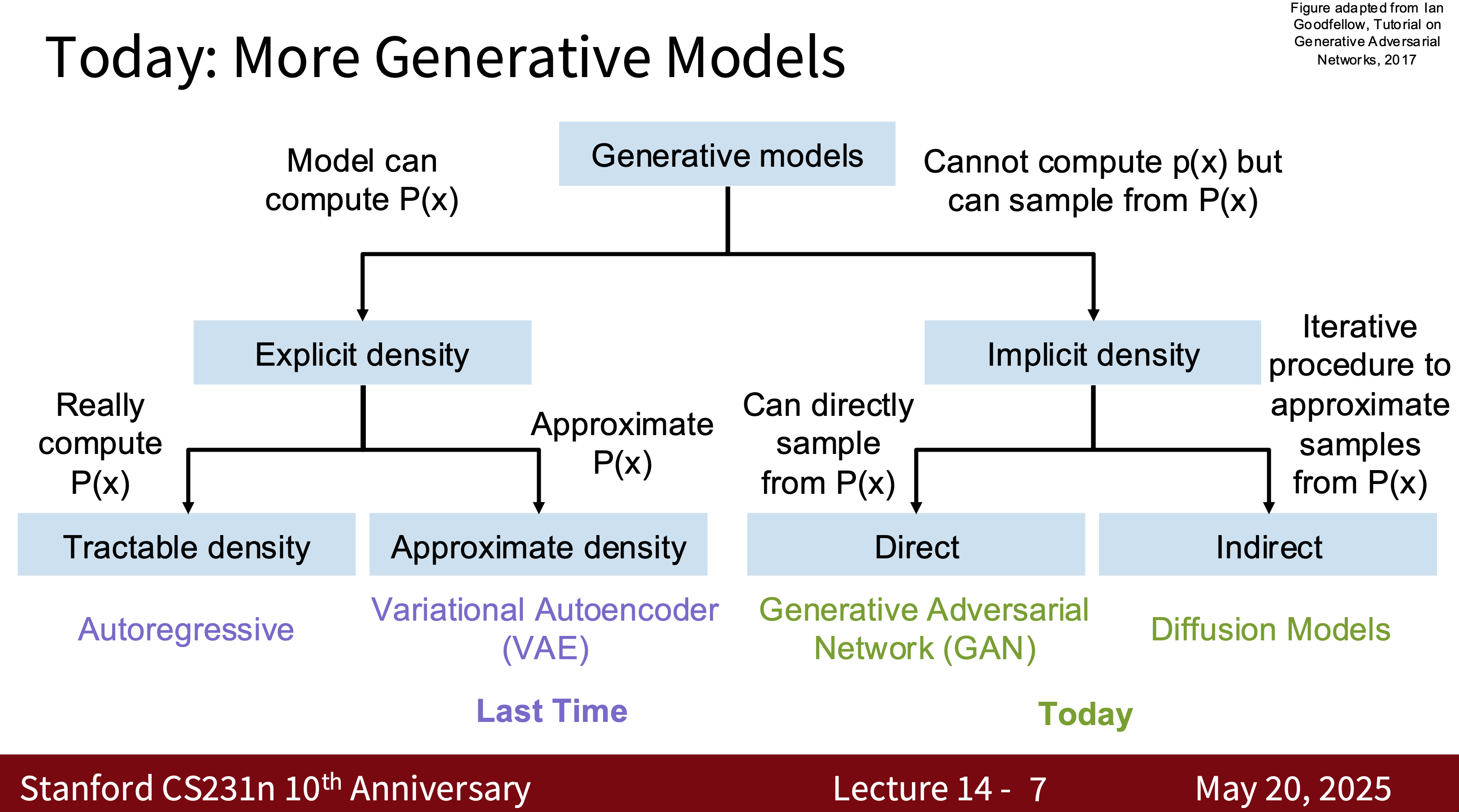
Deep Generative Models

What is a Deep Generative Model?
It learns the probability distribution $P(x)$ or conditional distribution $P(x \mid y)$ of the data and generates new samples similar to the training data.
Autoregressive Models, Energy-Based Models (EBM)
Image Generation: GAN, VAE, Diffusion Model
Text Generation (GPT Series)
Data Augmentation and Simulation
I know very little about deep generative models, but if you want to delve deeper, the best resources and lecture notes are cs236 and cs231n

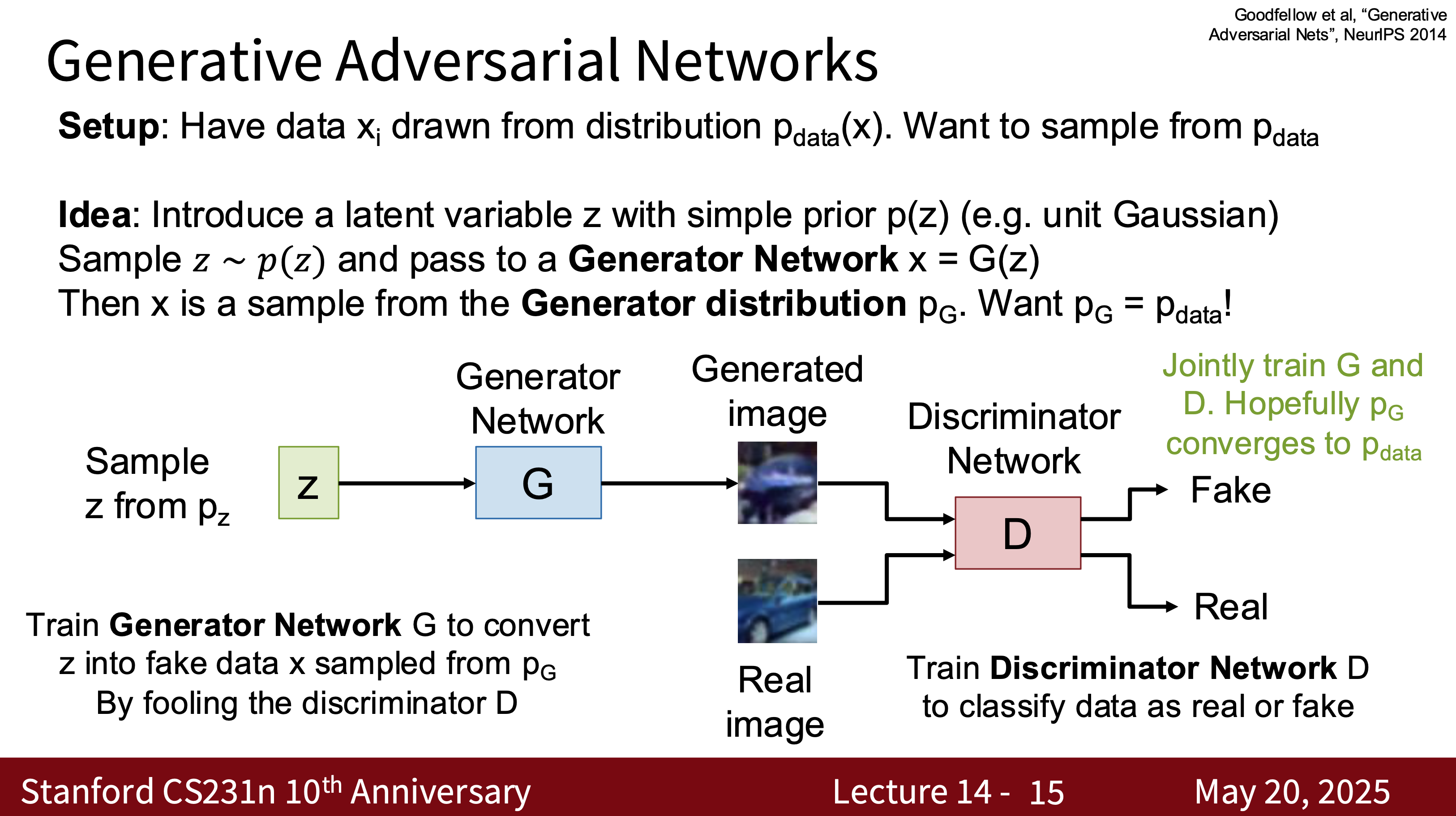
GAN

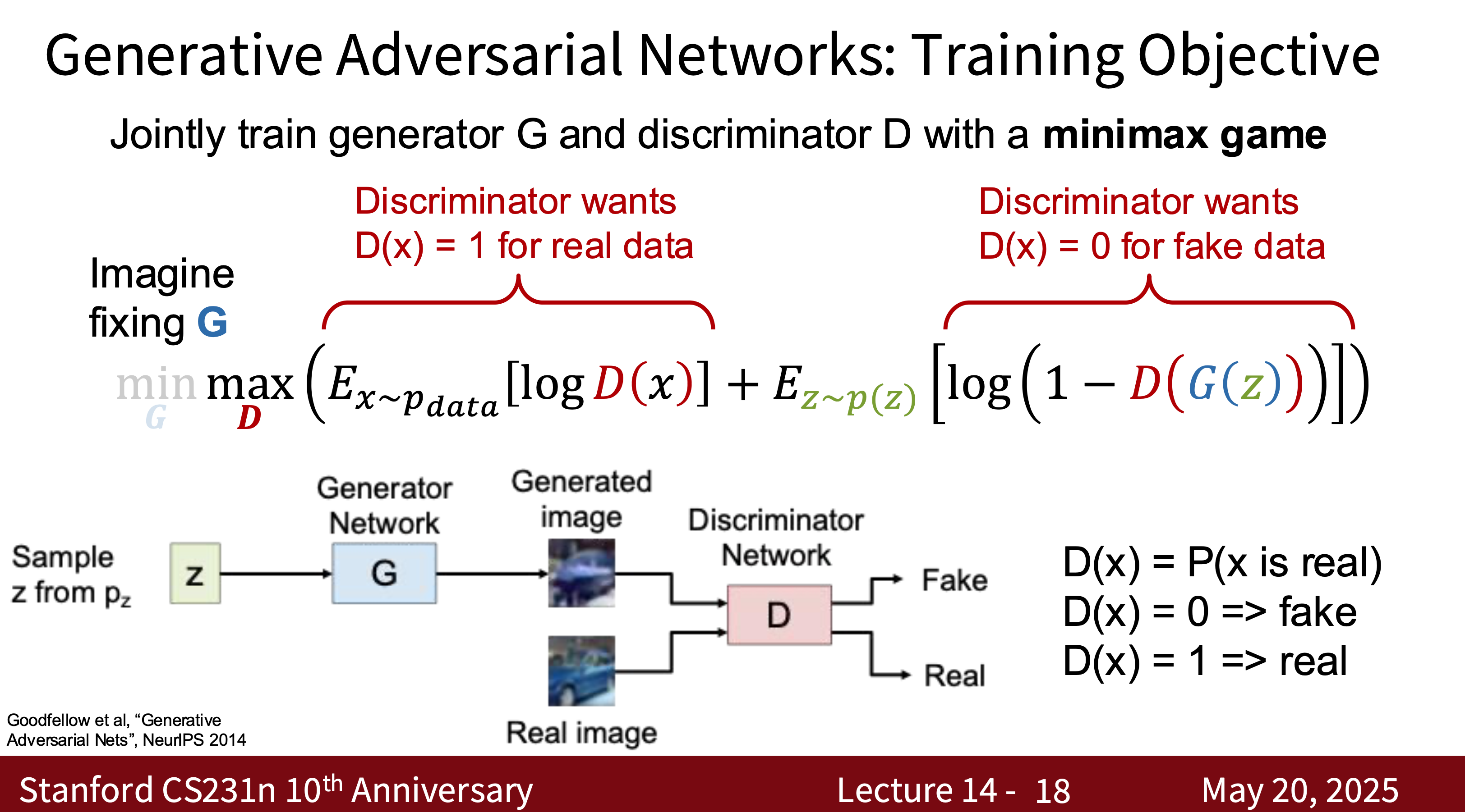
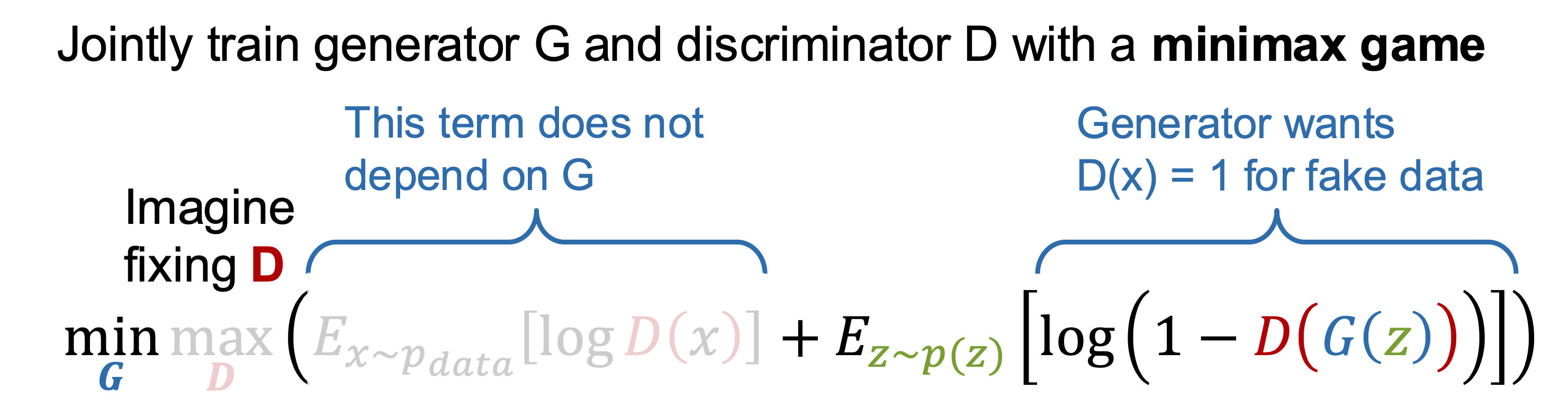
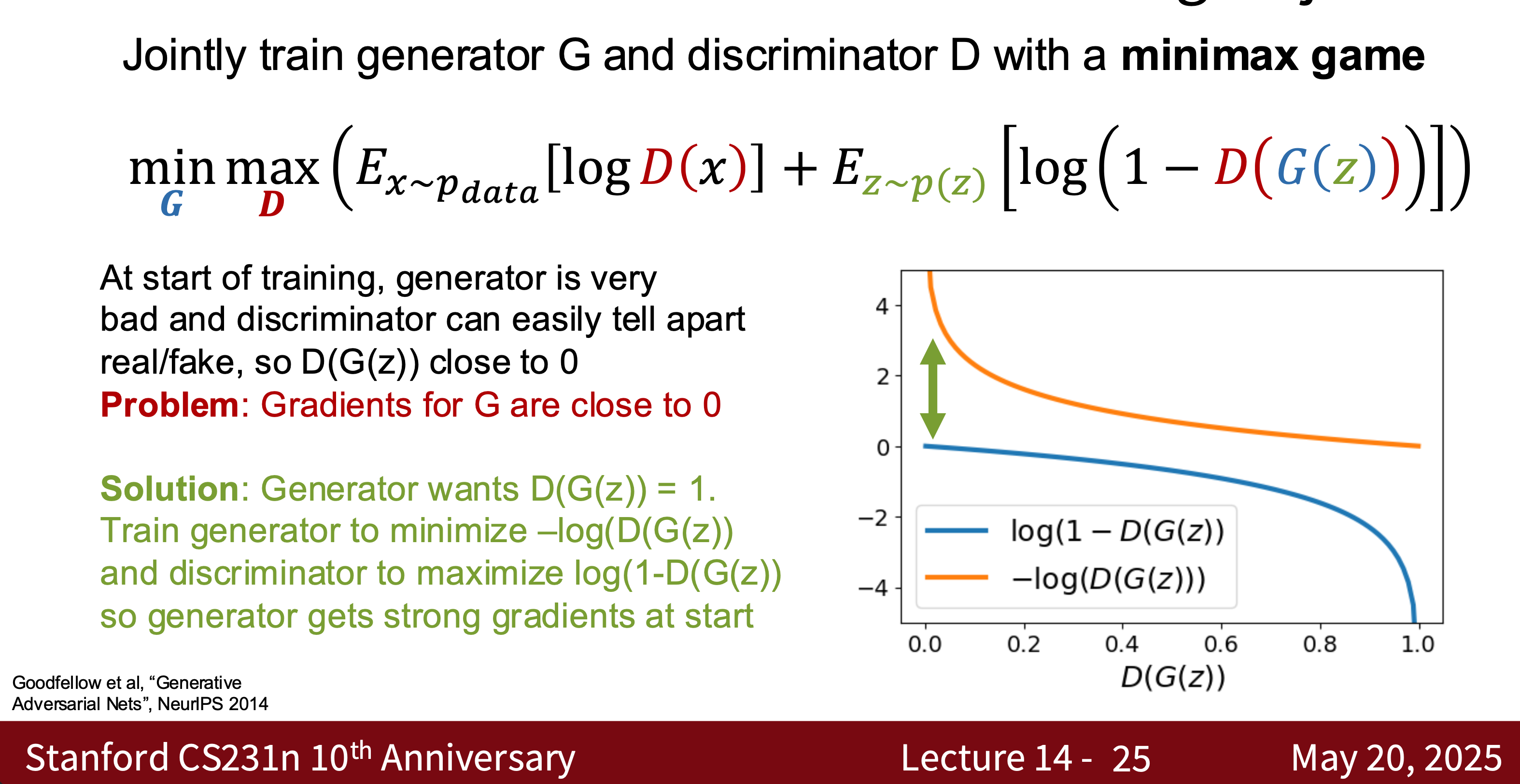
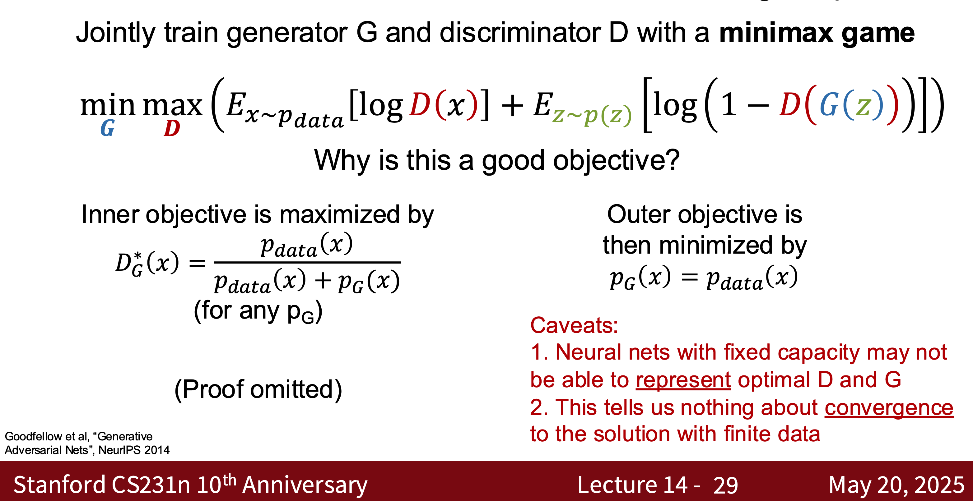
Training Two Networks—Generator $G$ and Discriminator $D$
Goal: $\min_G \max_D \mathbb{E}_{x \sim p_\text{data}}[\log D(x)] + \mathbb{E}_{z \sim p_z}[\log (1 - D(G(z)))]$
GAN variants include CD-GAN and Style-GAN. The difficulty in training GANs lies in the balance between the generator and the discriminator.

Training Step

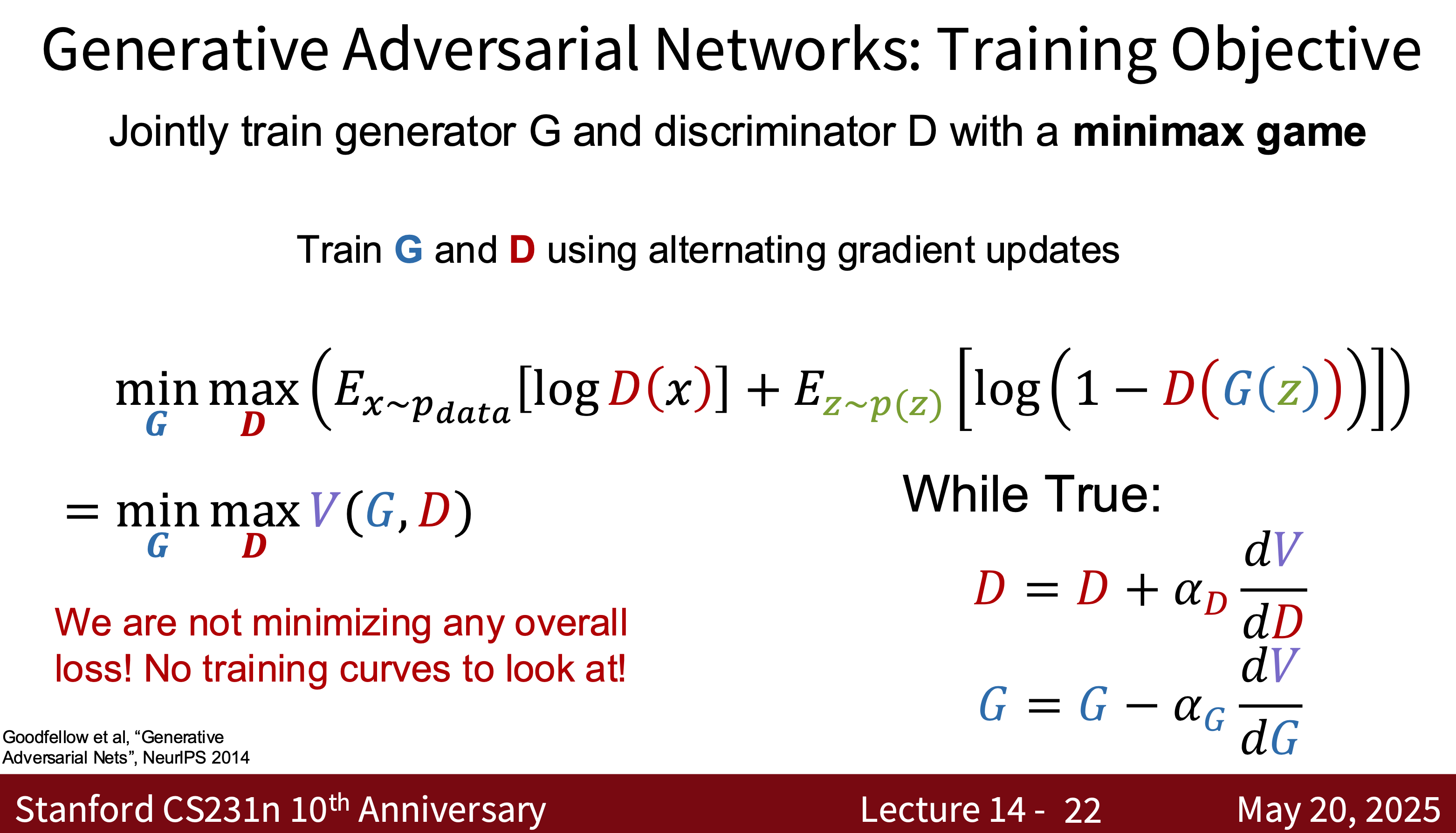
Some Questions with the Training Model

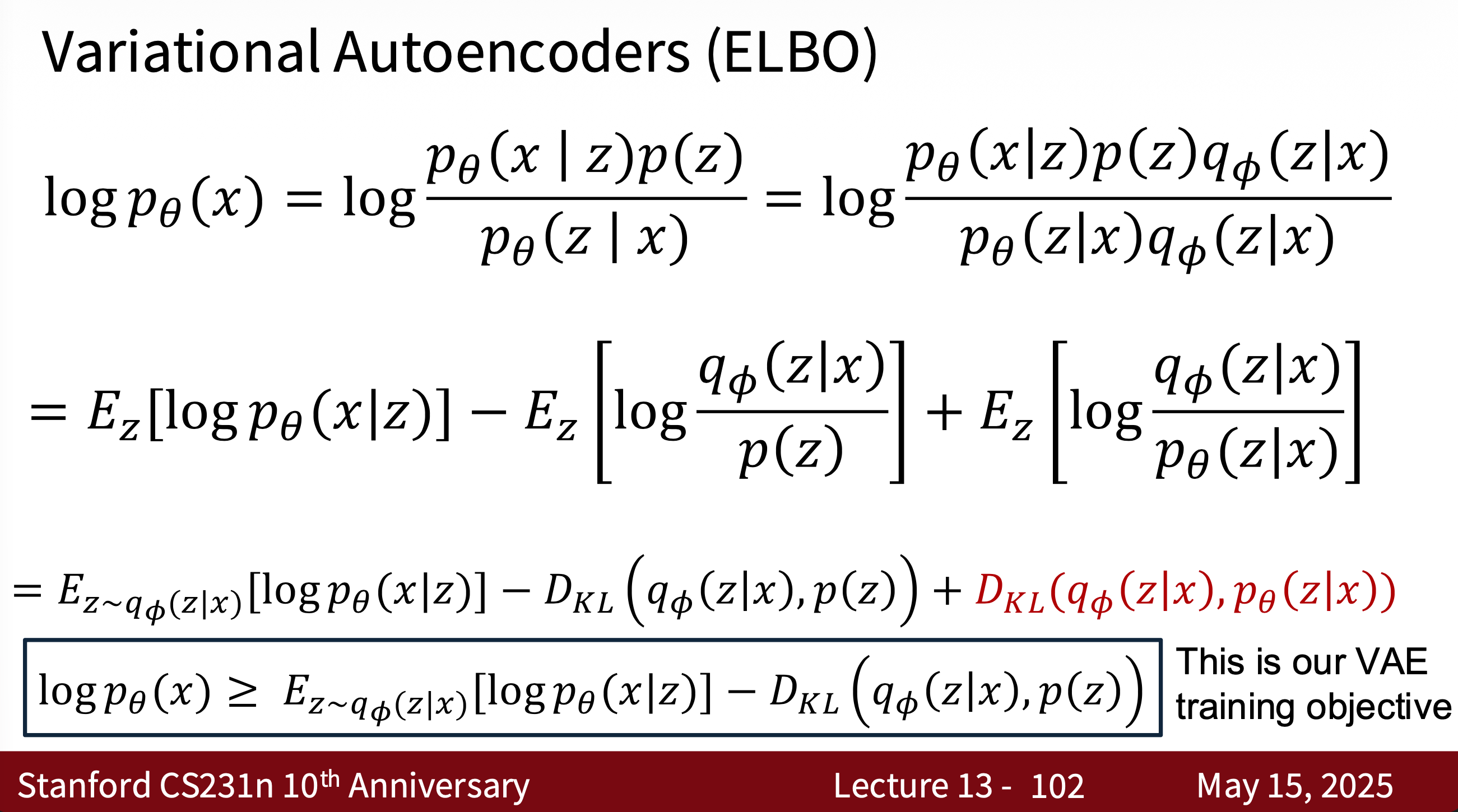
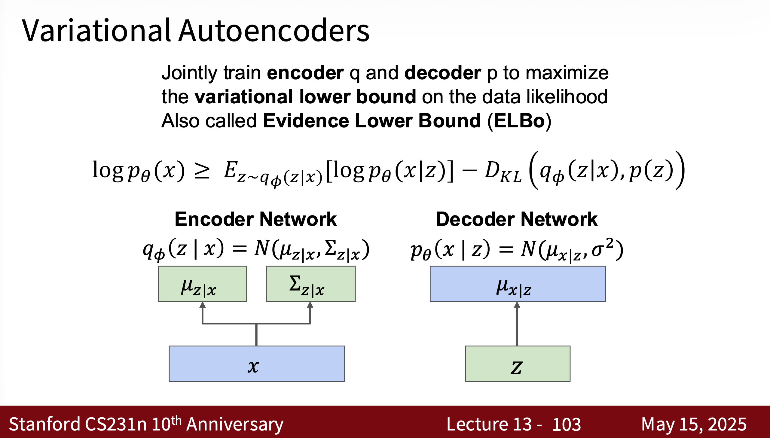
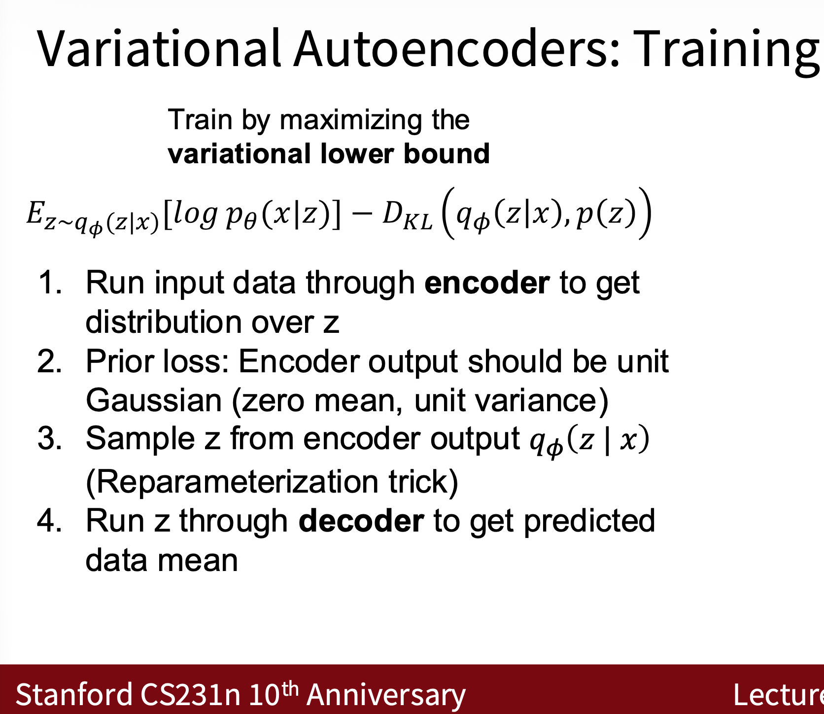
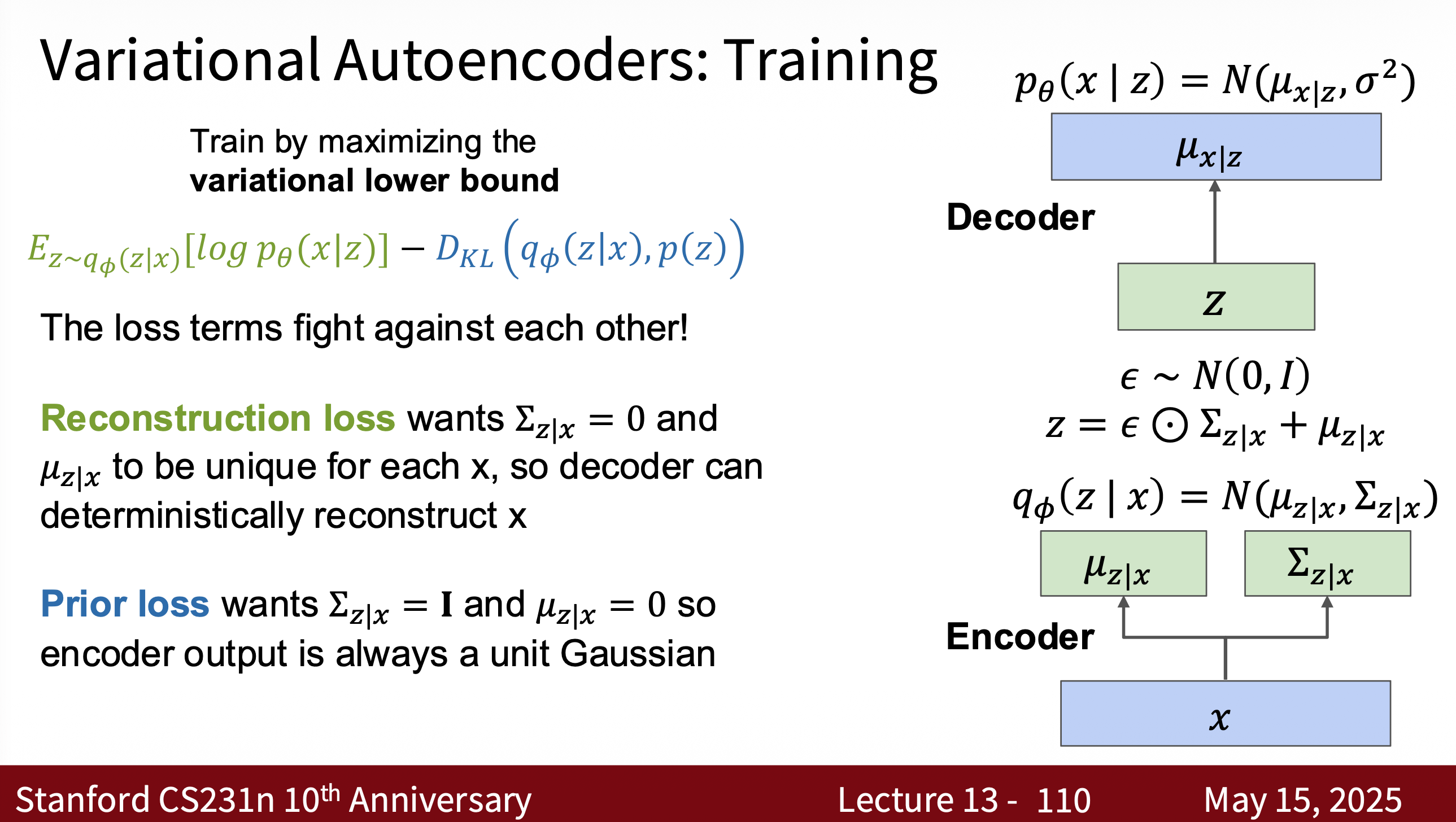
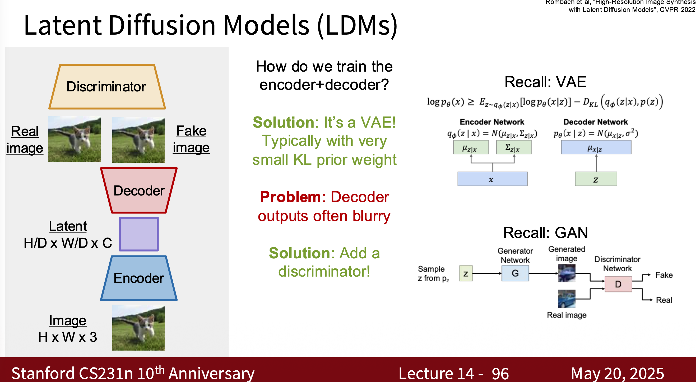
VAE

Maps data to a latent space $z$ and then reconstructs data from the latent space
Encoder: $q_\phi(z \mid x)$
Decoder: $p_\theta(x \mid z)$
Goal (ELBO): $\mathcal{L}(\theta, \phi; x) = \mathbb{E}_{q_\phi(z \mid x)}[\log p_\theta(x \mid z)] - \text{KL}(q_\phi(z \mid x) \| p(z))$
One of the best lectures on this topic is cs231n

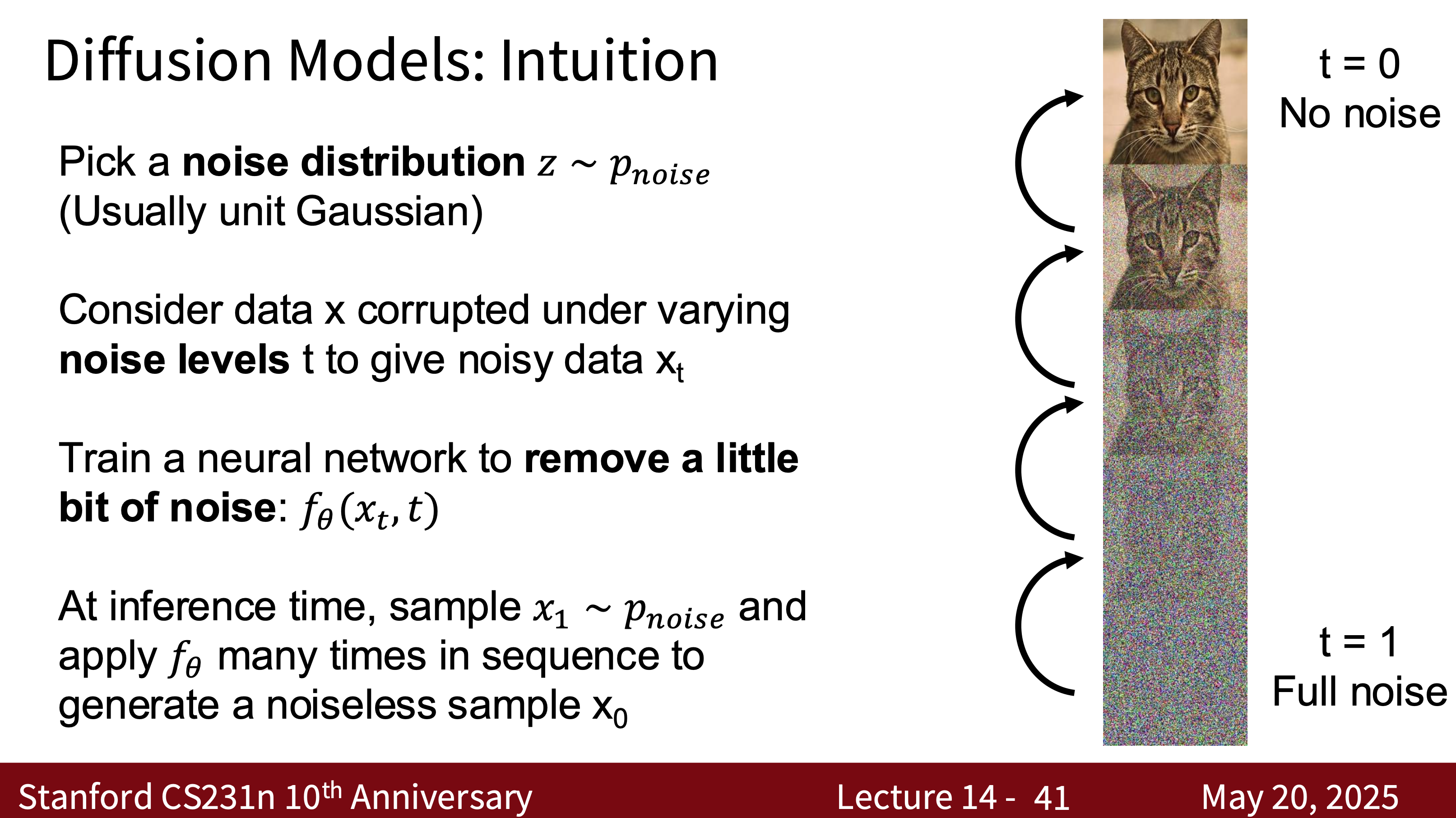
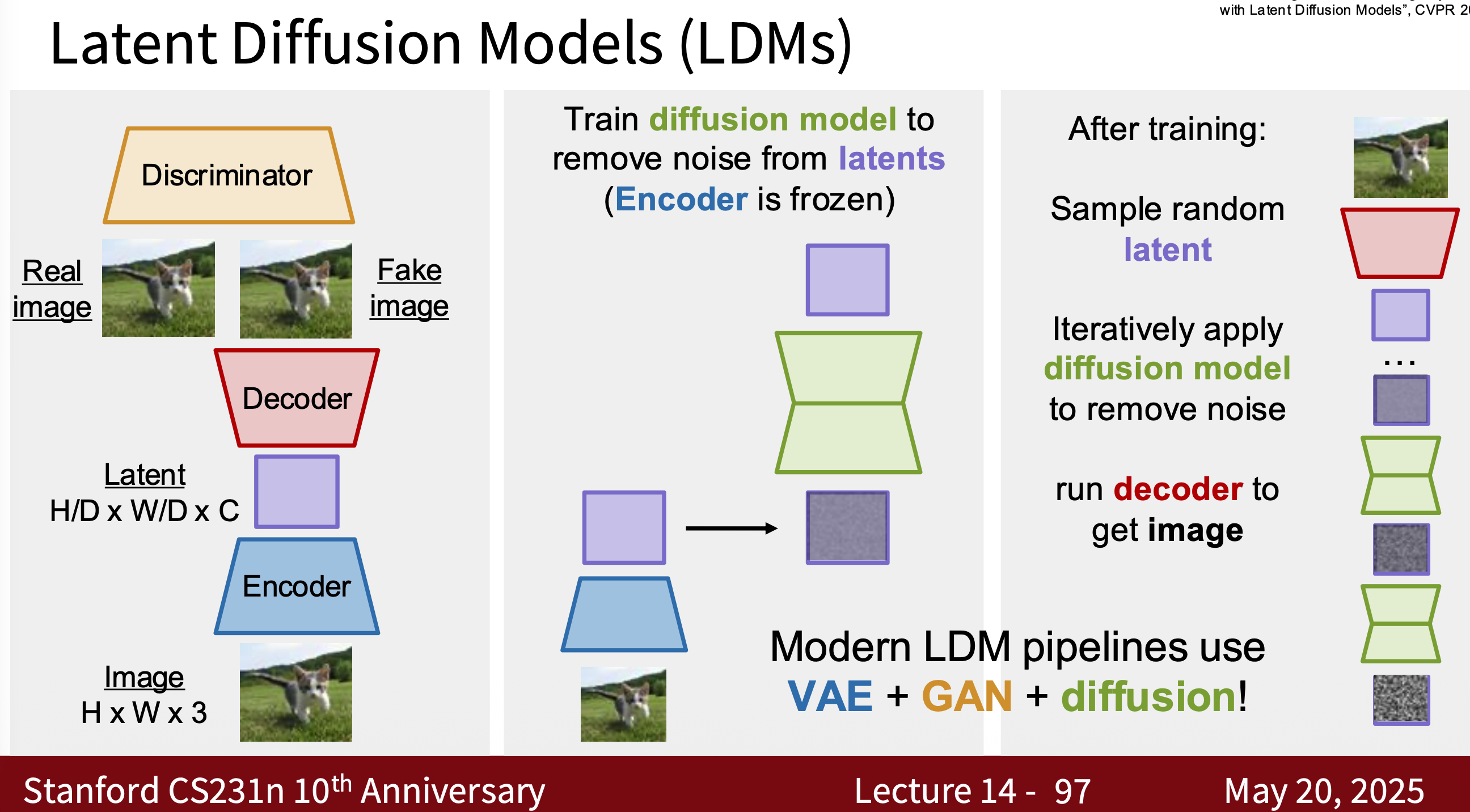
Diffusion Model

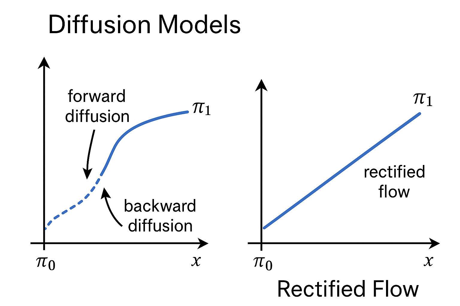
Generates samples by gradually adding noise to the data and then learning the inverse process of removing the noise.
Diffusion This model is also useful for generating text code for NLP. Some progress has been made. For details, please refer to the Google paper.
Forward (+noise): $q(x_t \mid x_{t-1})$
Backward (-noise): Learning $p_\theta(x_{t-1} \mid x_t)$
Goal (ELBO) $\mathcal{L}_{\text{ELBO}} = \mathbb{E} \Big[ \sum_{t=1}^T D_{KL}(q(x_t \mid x_{t-1}) \| p_\theta(x_{t-1} \mid x_t)) \Big]$
Diffusion models are a complex class of models. According to the instructor of cs231n, there are three different mathematical formulations for derivation.derivation and notation, and a 5-page derivation
Lilian weng’s blog
Sander Dielman’s blog -Some Paper:
High-level Overview

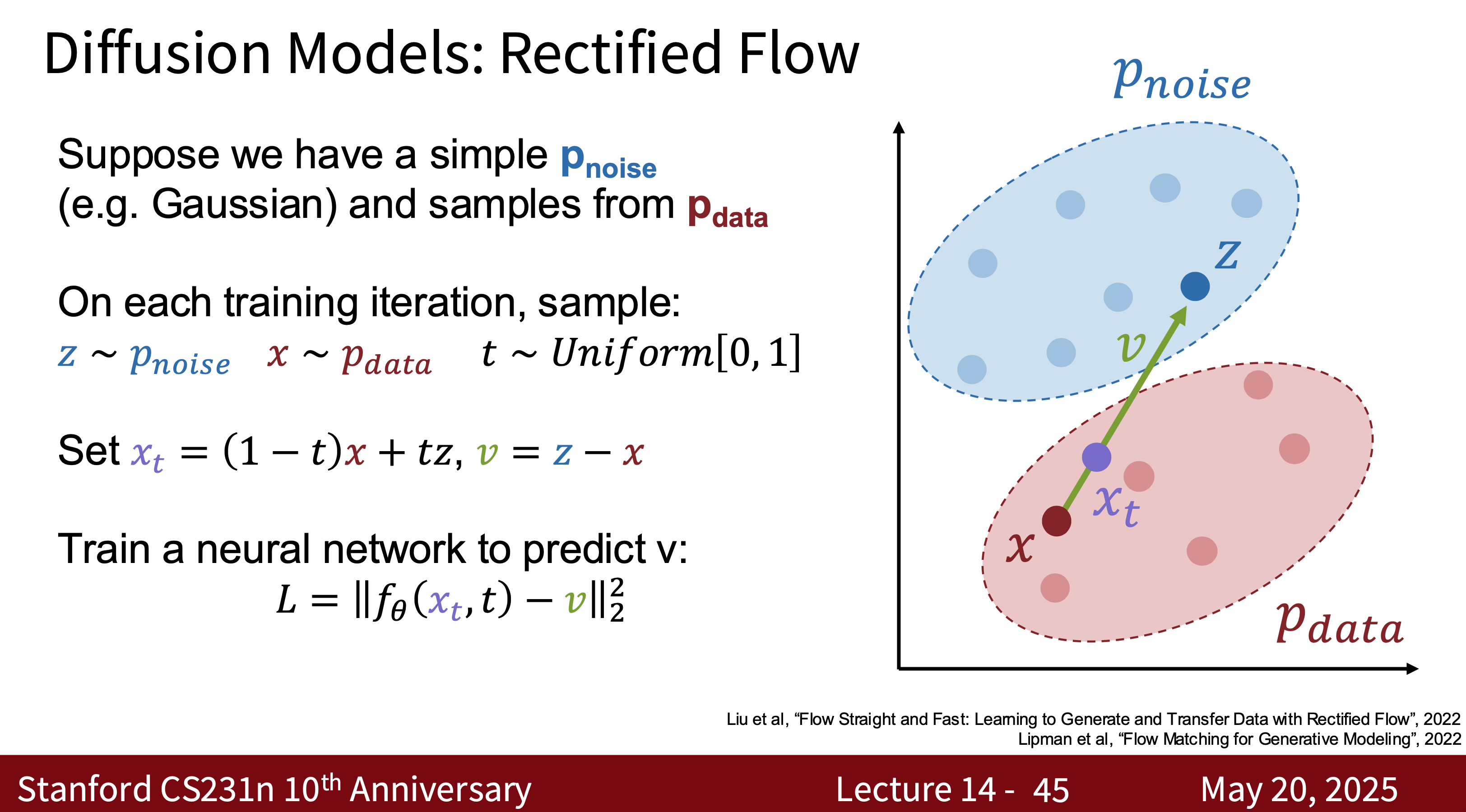
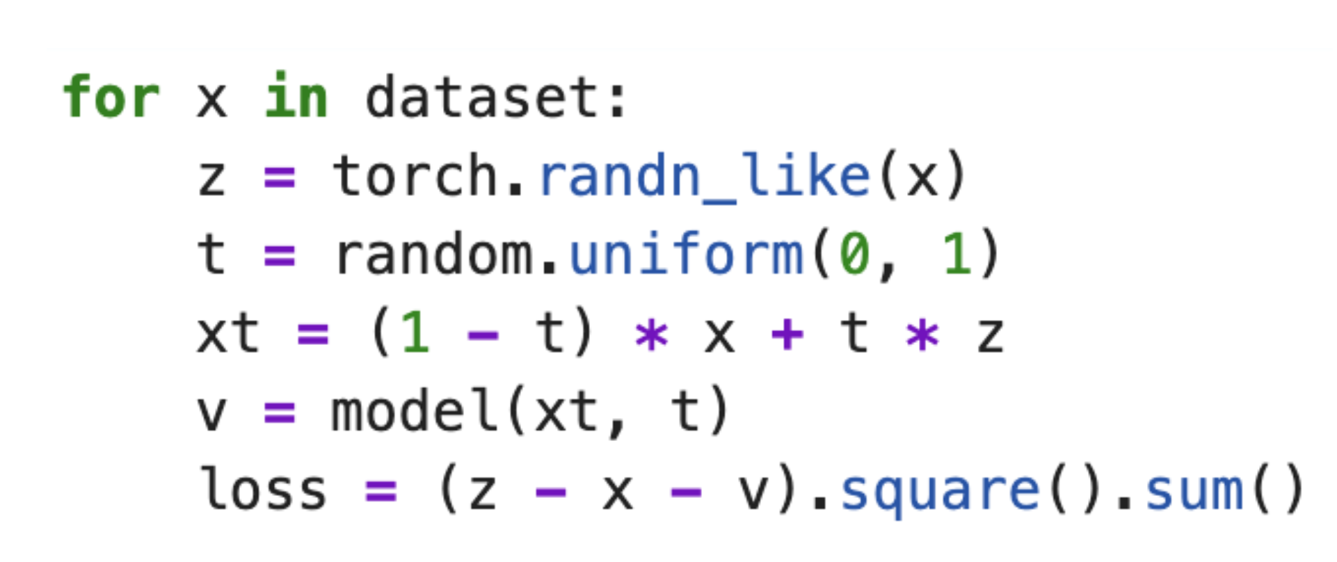
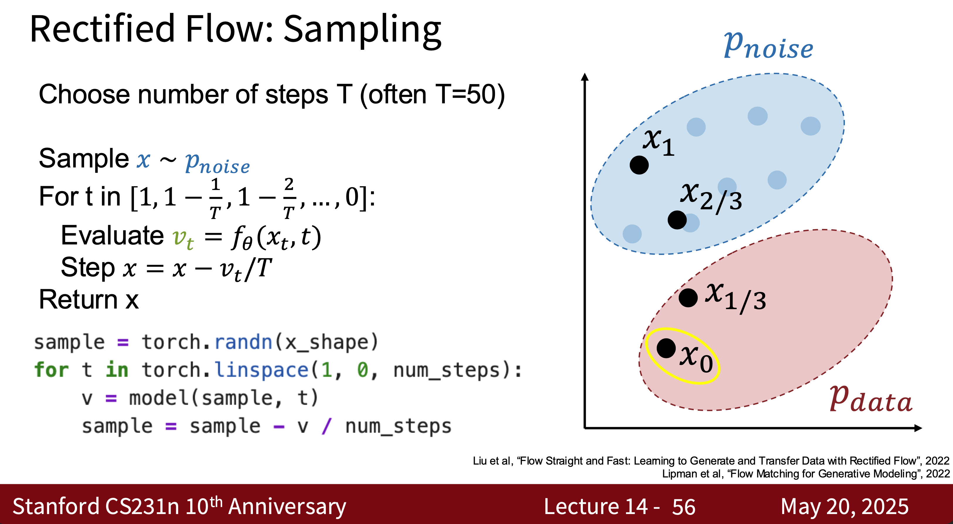
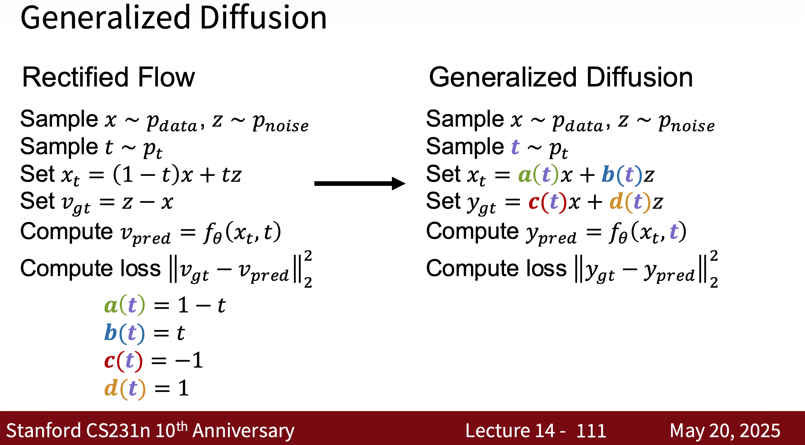
Intuitively, rectified flow models are a type of diffusion model.

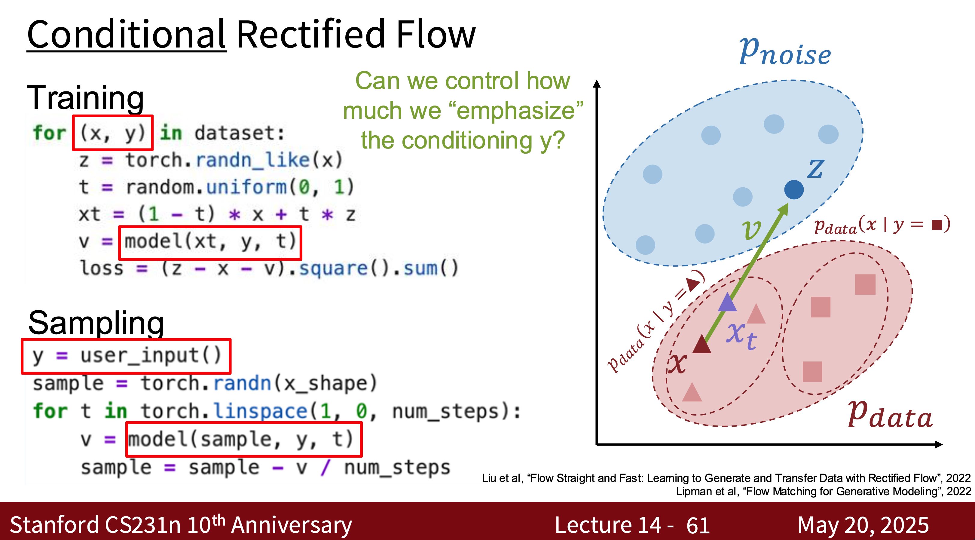
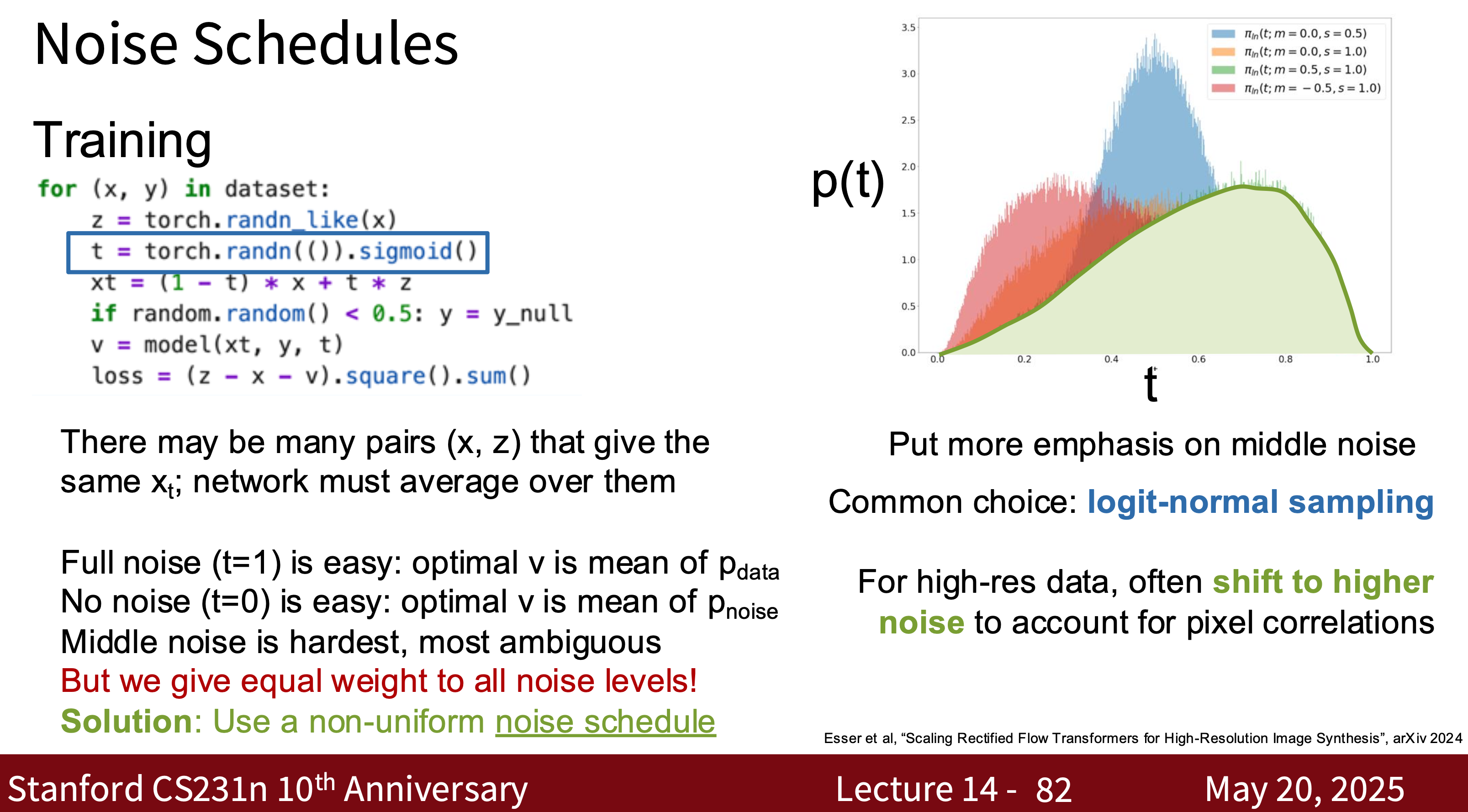
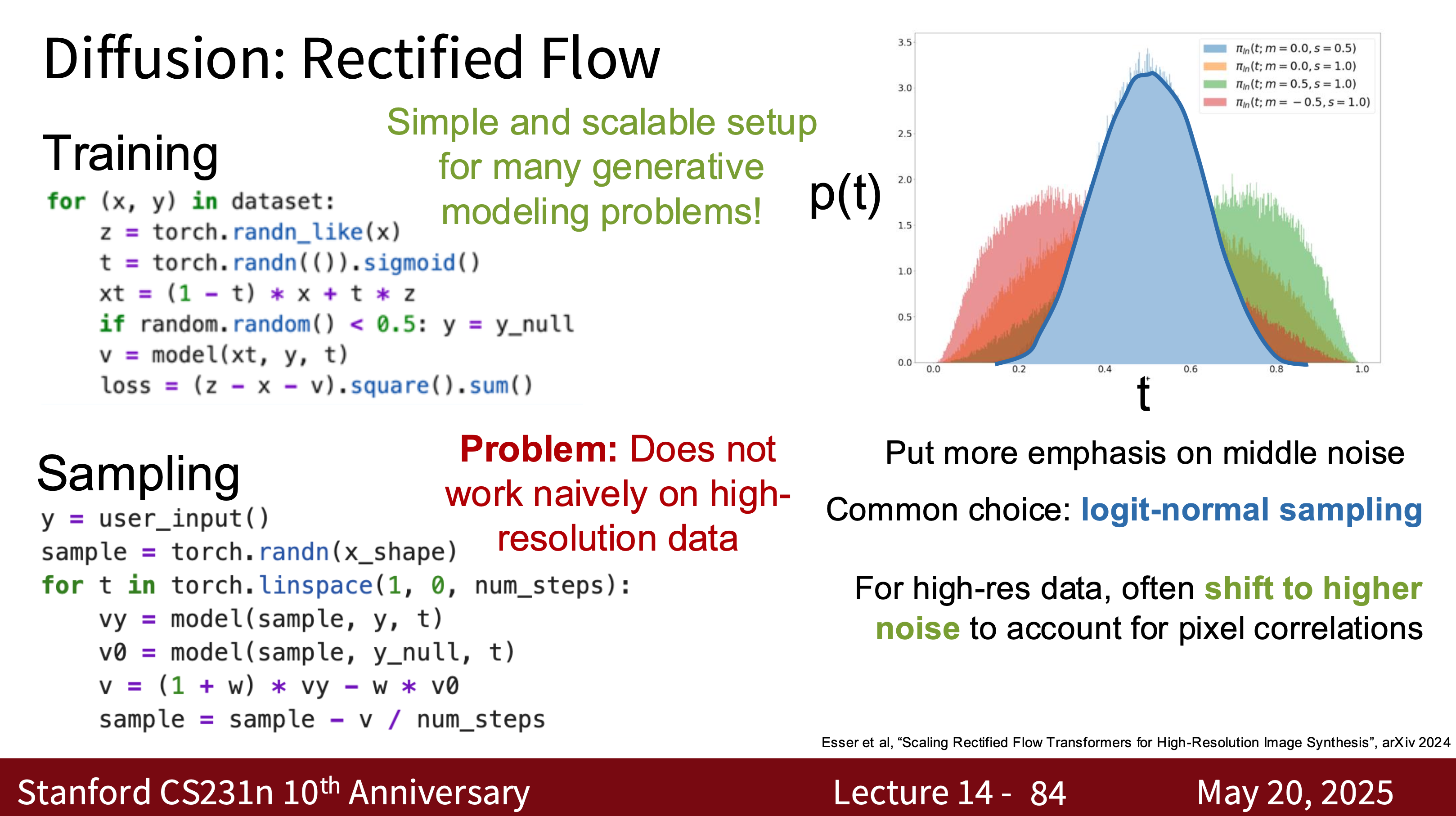
Modern Diffusion Model The most common one is Latent Diffusion Model (LDM) is essentially a combination of VAE, GAN, and Diffusion. Why? Because using modern diffusion models for tasks requires high-quality, well-generated data, which is the advantage of GANs. They can quickly generate latent spaces, which is the advantage of VAEs.

Diffusion transformer

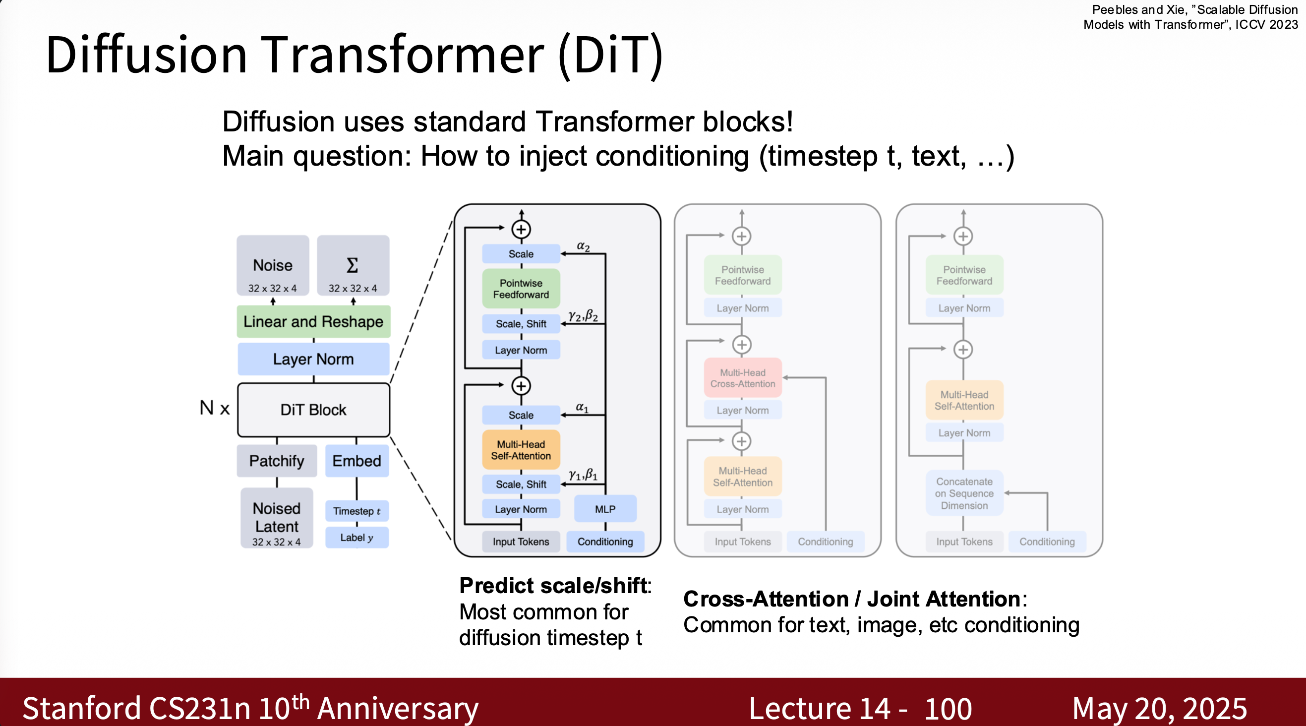
Some examples

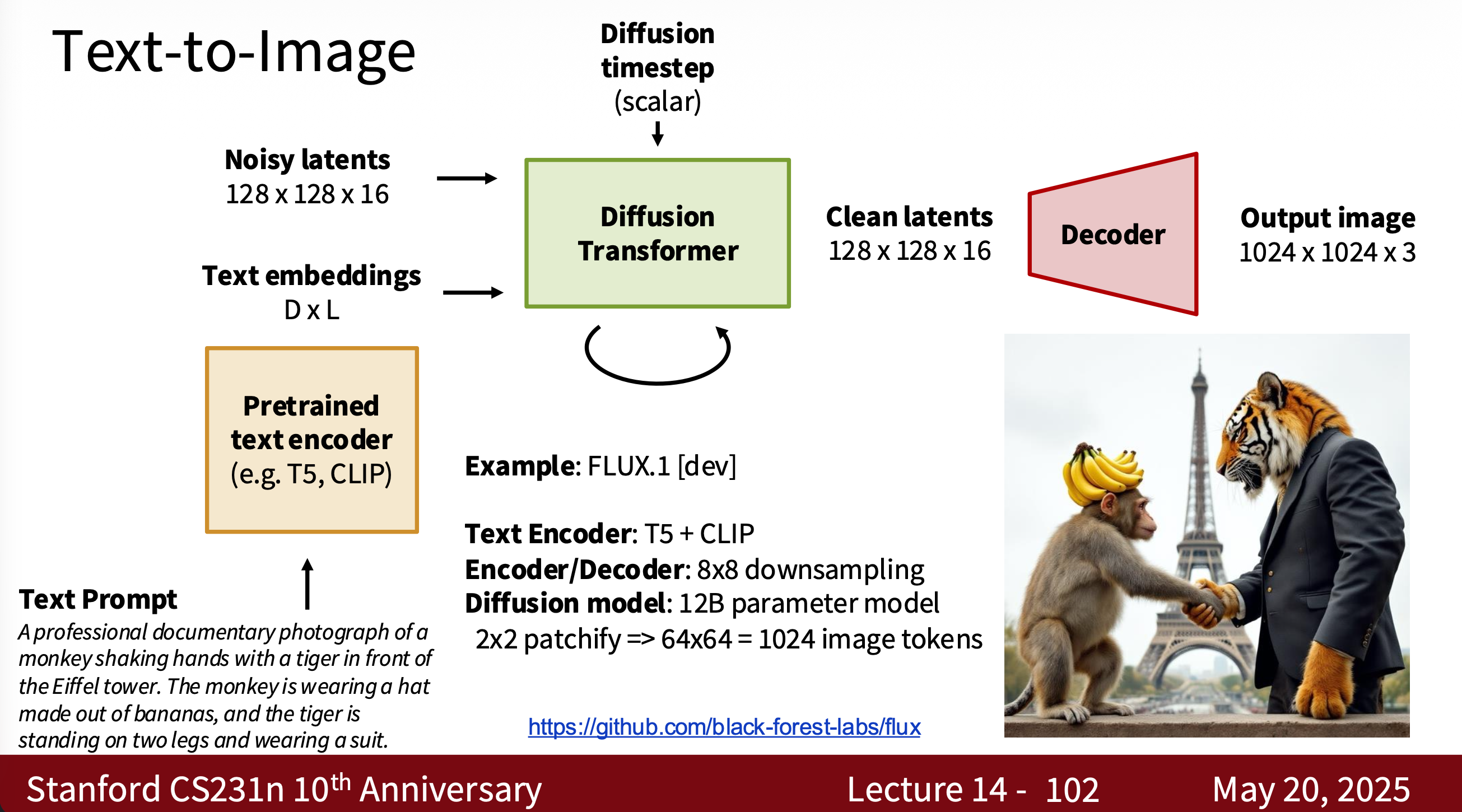
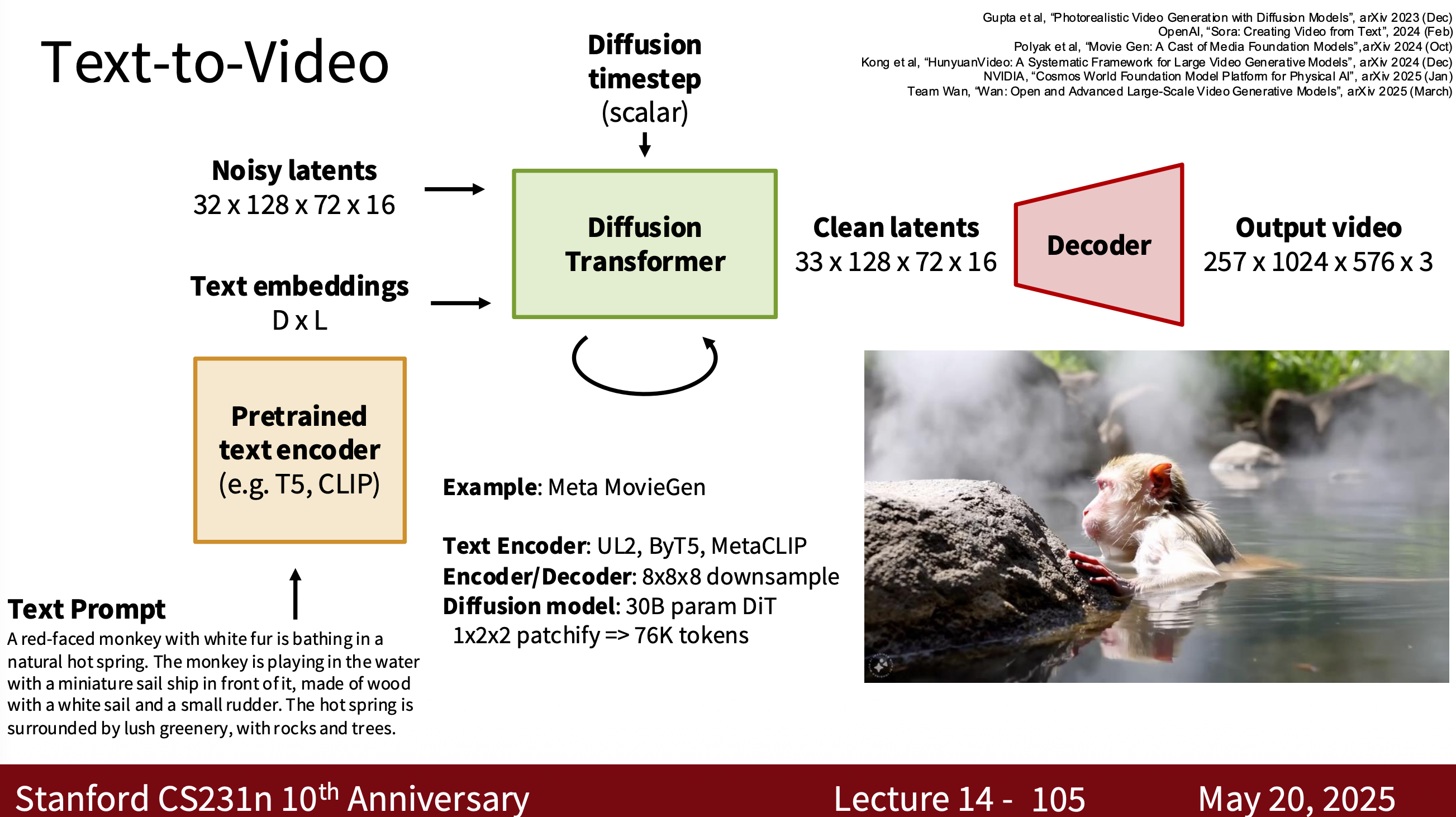
…For details, please see cs231n Lecture 14.

LLM Inference

We typically use Softmax to determine the probability of each token in the vocabulary, select the one with the highest probability (greedy search) and output it (using Tokenizer decode() to decode the token ID into a token). This token ID is then fed back into the model to predict the next token, looping until $$ is generated or the maximum length is reached (the maximum number of tokens output is typically set in config.yaml, for example, 2048 tokens). This step is typically called autoregression.
If the maximum number of tokens output is not set, issues such as increased latency, increased GPU memory usage, and duplicate model output can occur.
For multimodal LMs, such as images, the output tokens are typically latent codes, which are converted back to pixel images by the Decoder.
The vector dimensions of visual and textual tokens must be consistent to be able to be placed in the same Transformer.
To speed up inference, we typically use a KV Cache.
The core of the KV Cache technique is to store the key-value pairs (KVs) calculated after each attention layer is computed. This saved KV is then used each time the model is inferred, rather than recalculating the previous KVs. Cache:

cache[layer].k = [k1, k_k_new]
cache[layer].v = [v1, v_new]

Without using a KV cache, the time complexity is $O(N^{2} \cdot d)$. With a KV cache, the time complexity is reduced to $O(N \cdot d)$.
We typically use open-source libraries for LM output (HuggingFace Transformer, Ollama, etc.). This allows for generating a token and immediately returning it to the front-end interface or CLI. We call this step token-by-token streaming.
vLLM=>very fast LLM. This is an open-source inference engine specifically designed for LLM inference acceleration, supporting multi-user and high-concurrency scenarios. Its core technology is PageAttention, which addresses the problems of traditional KV caches: video memory fragmentation and memory waste. vLLM stores the KV cache as pages, rather than arrays. We can think of it as KV The cache implements “Virtual Memory” to support high concurrency. Compared to traditional one-shot batching, it can be interleaved, resulting in significantly higher concurrent throughput.
From a time complexity perspective, for an autoregressive model, the total complexity is $O(L \cdot N^{3} \cdot d)$, where L is the number of layers, N is the input sequence length, and d is the hidden dimension. Using only the KV Cache reduces the complexity to $O(L \cdot N^{2} \cdot d)$. Adding vLLM significantly reduces memory usage, while maintaining the overall complexity. Because P « N, vLLM only caches active pages, resulting in a memory usage of $P \times L \times d$, rather than the previous $N \times L \times d$.