Policy Gradient
-
Derivation of Policy Gradient
-
The goal of reinforcement learning is to maximize reward $r$. The policy $\pi$ is defined as selecting the optimal action to maximize $r$.
-
Policy Gradient is a method that directly adjusts the Action Method (Policy) to maximize reward.
-
In Policy Gradient, our goal is to optimize the policy \(\pi(a \mid s,\theta)\) to perform actions with higher rewards.
We aim to maximize an objective function \(J(\theta)\), which is typically the expected cumulative reward of the agent after executing policy \(\pi\).
\[J(\theta) = \mathbb{E}_{\tau \sim \pi_\theta} \left[ \sum_{t=0}^\infty \gamma^t r_t \right]\]Our Policy Gradient theorem is
\[\nabla J(\theta) \propto \sum_{s} \mu(s) \sum_{a} q_\pi(s,a)\, \nabla_\theta \pi(a|s,\theta)\]-
$\nabla J(\theta)$ is the gradient of policy performance with respect to parameters.
-
$\propto$ is proportional to, in simple terms, it’s either directly proportional or inversely proportional; variable x increases or decreases along with x.
-
$\sum_{s} \mu(s)$ is the robust distribution (state visitation frequency) of state $s$ under policy $\pi$, representing “how frequently the agent visits state s” in the long run. Sometimes it’s $\rho^\pi(s)$, but it’s the same; it’s a sampling probability used to weight the states.
\(\sum_a q_\pi(s,a) \nabla_{\theta} \pi(a|s,\theta)\)
-
is a weighted average of all possible actions \(a\) for each state \(s\).
-
$q_\pi(s,a)$ in state s Expected reward (Q-value) after performing action a.
\(\nabla_{\theta} \pi(a|s,\theta)\)
- is the gradient of the policy function with respect to the parameters, representing “how to fine-tune the parameters to increase the probability of the action”.
Proof of our Policy Gradient Theorem (episodic case, from Sutton textbook)
- The state-value function can be represented in the form of an action-value function.
- The probability that we transition from state s to state x.
Policy gradient methods generally include
- Policy gradient classification includes On-policy, Off-policy, and Iteration.
- On-policy must be sampled from the current policy $\pi_{\theta}$.
- Off-policy allows sampling from other policies $\mu$ to update the policy $\pi$.
-
In \(\nabla_{\theta} J(\theta) = \mathbb{E}_{\tau \sim \mu}\left[\frac{\pi_{\theta}(a|s)}{\mu(a|s)} \nabla_{\theta} \log \pi_{\theta}(a|s) \, G_t \right]\) ,the ratio \(\frac{\pi_{\theta}}{\mu}\) belongs to importance sampling (IS).
- Importance Sampling is a general method in probability theory used to calculate the expectation of a target distribution $p$, but the samples come from another distribution $q$.
In \(\mathbb{E}_{x \sim p}[f(x)] = \mathbb{E}_{x \sim q}\left[\frac{p(x)}{q(x)} f(x)\right]\),
\(\rho(x) = \frac{p(x)}{q(x)}\) are the IS weights. - Iteration refers to both the concept of policy iteration (evaluation + improvement) and the mini-batch multi-round updates in actual implementation.
- The most basic REINFORCE method uses Monte Carlo sampling estimation.
- REINFORCE with Baseline introduces a baseline to reduce variance.
-
Actor-Critic method: the policy function is used to select actions, and the value function is used to evaluate their quality.
- Proximal Policy Optimization (PPO) Algorithm
- Direct Preference Optimization (DPO) Algorithm
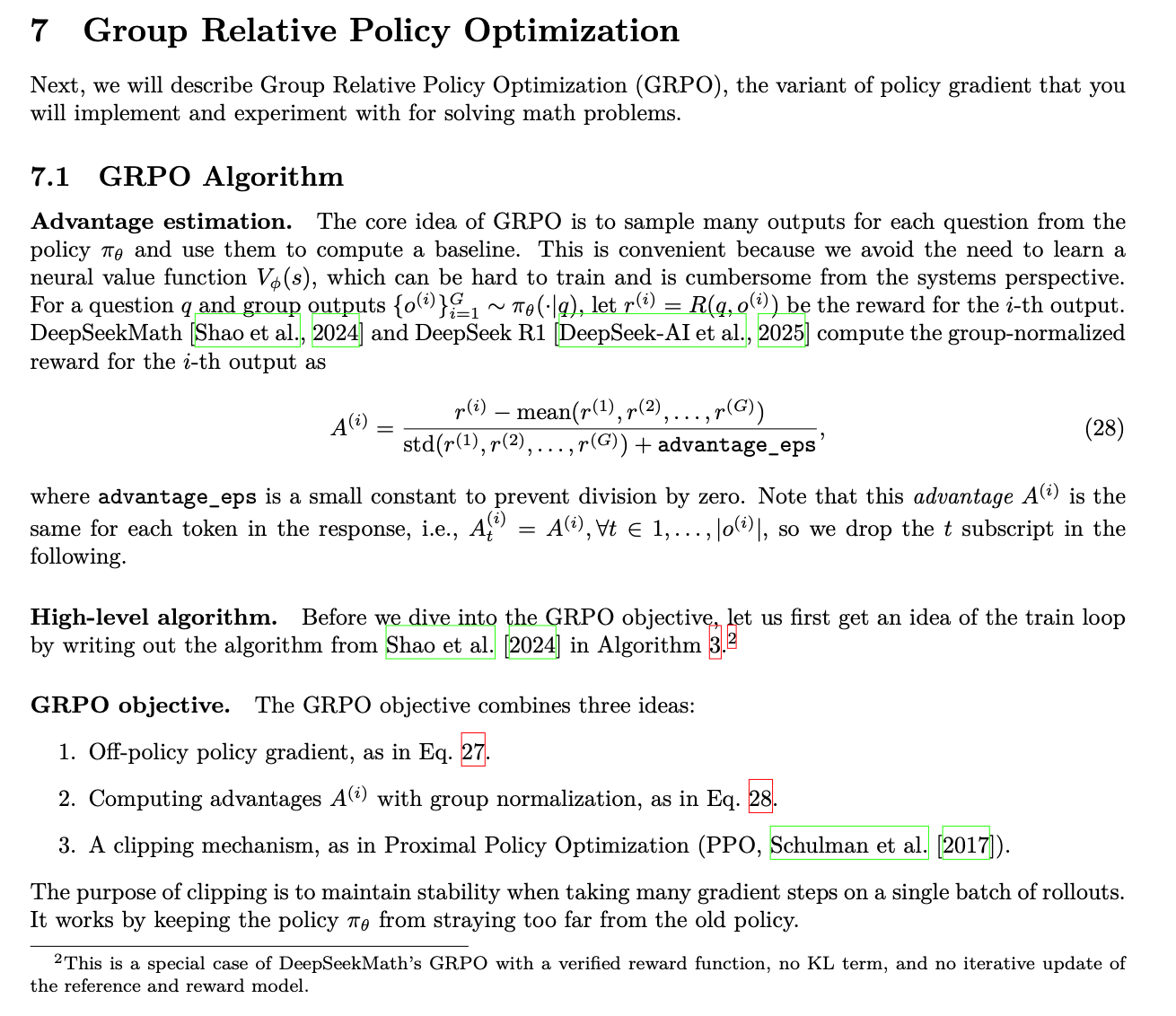
- Group Relative Policy Optimization (GRPO) (DeepSeek R1), etc.
-
Eligibility Traces are temporal credit assignment mechanisms (TD(λ), Actor-Critic(λ)), making gradients propagate more smoothly over time.
In Deep RL, we usually use GAE (Generalized Advantage Estimation) instead. - When implementing these algorithms, we distinguish between episodic (with an end, e.g. games) and continuing (without an end, infinite).
The focus here is on PPO, DPO, and GRPO.
REINFORCE
\[\nabla J(\theta) \propto \sum_{s} \mu(s) \sum_{a} q_{\pi}(s,a)\, \nabla_{\theta} \pi(a|s,\theta) = \mathbb{E}\left[\sum_{a} q_{\pi}(S_t,a) \nabla_{\theta} \pi(a|S_t,\theta)\right] \tag{13.6}\]Gradient-Ascent Update Step: \(\theta_{t+1} := \theta_t + \alpha \sum_{a} \hat{q}(S_t,a,w)\, \nabla_{\theta} \pi(a|S_t,\theta)\)
From (13.6), we deduce the sampling form: \(\begin{aligned} J(\theta) &= \mathbb{E}_{\pi} \left[ \sum_a \pi(a|S_t,\theta) q_{\pi}(S_t,a)\frac{\nabla_{\theta} \pi(a|S_t,\theta)}{\pi(a|S_t,\theta)} \right] \\ &= \mathbb{E}_{\pi} \left[ q_{\pi}(S_t,A_t)\frac{\nabla_{\theta} \pi(A_t|S_t,\theta)}{\pi(A_t|S_t,\theta)} \right] \quad \text{(replace $a$ with sampled $A_t$)} \\ &= \mathbb{E}_{\pi} \left[G_t \frac{\nabla_{\theta} \pi(A_t|S_t,\theta)}{\pi(A_t|S_t,\theta)} \right], \quad \text{where } \mathbb{E}_{\pi}[G_t|S_t,A_t]=q_{\pi}(S_t,A_t) \end{aligned}\)
REINFORCE Update: \(\theta_{t+1} := \theta_t + \alpha\, G_t\, \frac{\nabla_{\theta} \pi(A_t|S_t,\theta)}{\pi(A_t|S_t,\theta)}\)
REINFORCE with Baseline
\[\nabla J(\theta) \propto \sum_{s} \mu(s) \sum_{a} \big(q_{\pi}(s,a) - b(s)\big)\, \nabla_{\theta} \pi(a|s,\theta)\]Update: \(\theta_{t+1} := \theta_t + \alpha\, \big(G_t - b(S_t)\big)\, \frac{\nabla_{\theta} \pi(A_t|S_t,\theta)}{\pi(A_t|S_t,\theta)}\)
Actor-Critic
From Sutton’s derivation, the update is: \(\begin{aligned} \theta_{t+1} &:= \theta_t + \alpha \big(G_{t:t+1} - \hat{v}(S_t, w)\big)\, \frac{\nabla_{\theta} \pi(A_t|S_t,\theta)}{\pi(A_t|S_t,\theta)} \\ &= \theta_t + \alpha \big(G_{t:t+1} - \gamma \hat{v}(S_{t+1},w) - \hat{v}(S_t,w)\big)\, \frac{\nabla_{\theta} \pi(A_t|S_t,\theta)}{\pi(A_t|S_t,\theta)} \\ &= \theta_t + \alpha\, \delta_t\, \frac{\nabla_{\theta} \pi(A_t|S_t,\theta)}{\pi(A_t|S_t,\theta)} \end{aligned}\)
Proximal Policy Optimization (PPO)
- Key idea: use a clipped surrogate objective to constrain large policy updates.
- Policy ratio:
$r_t(\theta) = \dfrac{\pi_{\theta}(a_t|s_t)}{\pi_{\text{old}}(a_t|s_t)}$ - PPO-Clip surrogate:
$L^{\text{CLIP}}(\theta) = \mathbb{E}_t\Big[\min\big(r_t(\theta)\hat{A}_t,\, \operatorname{clip}(r_t(\theta), 1-\epsilon, 1+\epsilon)\hat{A}_t\big)\Big]$ - GAE (Advantage Estimation):
\(\delta_t = r_t + \gamma V(s_{t+1}) - V(s_t), \quad \hat{A}_t = \sum_{l=0}^{\infty} (\gamma\lambda)^l \delta_{t+l}\) - Total loss (value + entropy regularization):
\(L(\theta) = -L^{\text{CLIP}}(\theta) + c_1\,\mathbb{E}_t\big[(V_{\theta}(s_t)-R_t)^2\big] - c_2\,\mathbb{E}_t\big[S[\pi_{\theta}](s_t)\big]\)
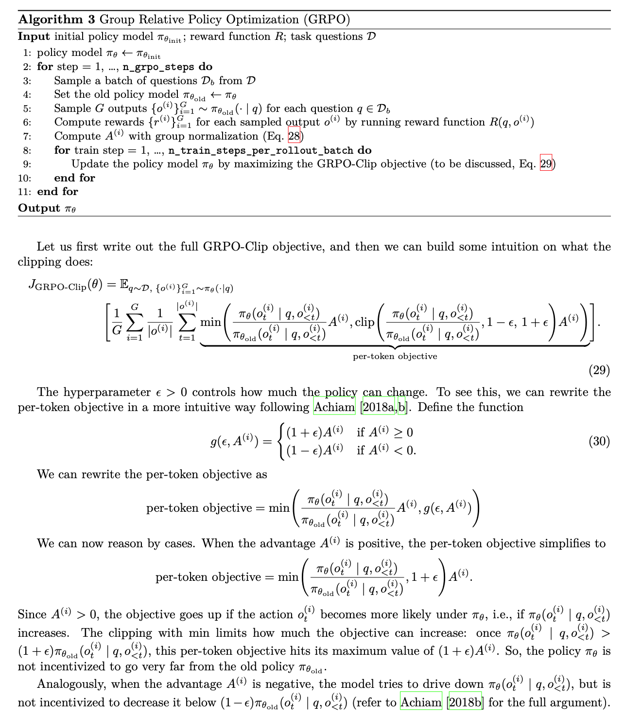
Group Relative Policy Optimization
Enjoy Reading This Article?
Here are some more articles you might like to read next: